Color coding rows in an Excel spreadsheet based on a specific cell value is a powerful way to organize and analyze your data at a glance. By applying different colors to entire rows according to the content of a single cell, you can quickly identify key information, track statuses, or highlight categories, making your spreadsheet easier to read and more efficient to use.
This article will walk you through the step-by-step process of setting up color-coded rows using Excel’s conditional formatting. The example begins with a spreadsheet that we created using drop-down cells. You can color-code rows based on any data within a cell, though.
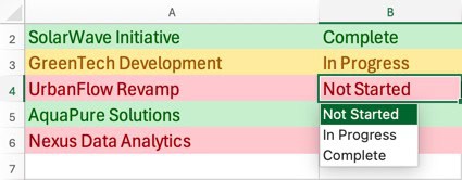
In this article, we’ll change the color of part of a row when a specific option is selected on the drop-down.
It’ll look something like this.
The screenshots and instructions are all on the Mac Microsoft 365 version of Excel. Some aspects of the process are similar to the Windows version, but it varies from steps 4 through 11. You may get lost in Windows if you’re not relatively familiar with Excel.
Open Conditional Formatting Rules Window
Step 1: Click the Home tab on the Excel ribbon.
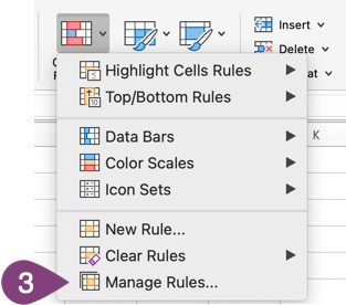
Step 2: Click the Conditional Formatting button.

Step 3: Select Manage Rules… from the drop-down.
Create a New Formatting Rule
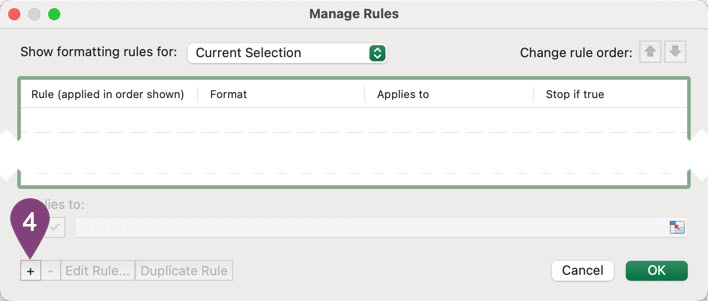
Step 4: Click the + button at the bottom of the Manage Rules window.
Step 5: Select Classic from the Style drop-down.
Step 6: Select Use a formula to determine which cells to format from the next drop-down so you can enter your own formula.
Step 7: Set the formula to the cell to format and the value it should equal to format it.

Why the formula in step 7 uses $B2 instead of $B$2:
In the image, we use $B2 instead of $B$2, but why?
When applying conditional formatting to multiple rows, you need the formula to check a different cell in column B for each row.
- $B2 (correct): The dollar sign before B locks the column to B, but leaves the row number flexible. So row 1 checks B1, row 2 checks B2, row 3 checks B3, and so on.
- $B$2 (incorrect): Both dollar signs lock the formula to only look at cell B2, no matter which row you’re formatting. This means every row would only check B2 for the “Complete” value, instead of checking its corresponding cell in column B.
The key principle: Use a dollar sign ($) before the column letter to keep it fixed, but leave the row number without a dollar sign so it adjusts automatically for each row being formatted.
This way, each row’s formatting is based on its own value in column B, not just a single fixed cell. You can learn more about absolute, relative, and mixed references on this Microsoft support article.
Step 8: Choose the format from the drop-down or set up a custom format.
Step 9: Click OK.
Select Which Cells The Formatting Rule Applies To
Step 10: Use the button on the right side of the Applies to: box to select which cells you’d like this rule to apply to.
We only wanted to change the color for columns A & B on the Projects sheet, but you can apply the color formatting to the entire row by not defining the row, which would look like =$1:$28 to cover rows 1 through 28. Just increase the 28 to whatever you want to color-code more rows.
Step 11: Click the green ✓ to save which cells the formatting applies to.
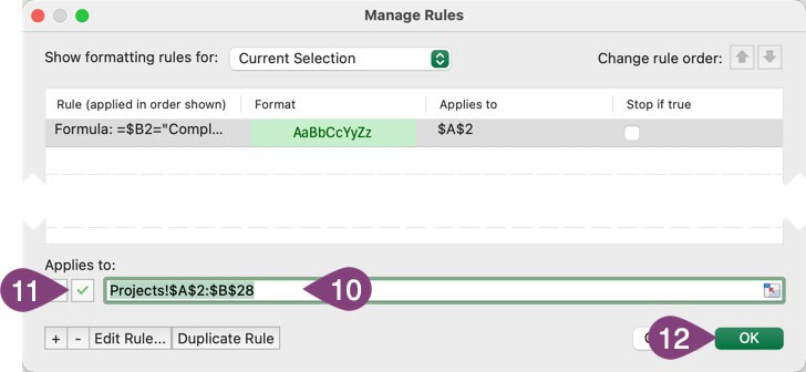
Step 12: Click OK.
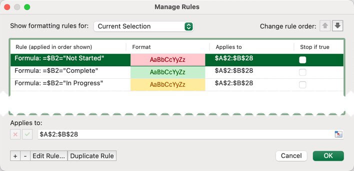
Now you have a formatting rule that will color-code the row (or portion of a row in our case) based on what is inserted in a specific cell. You can see that we duplicated the rule we created and assigned different colors based on whether you select ‘Not Started’, ‘Complete’, or ‘In Progress’ from the drop-down menu.
Here’s how it works.
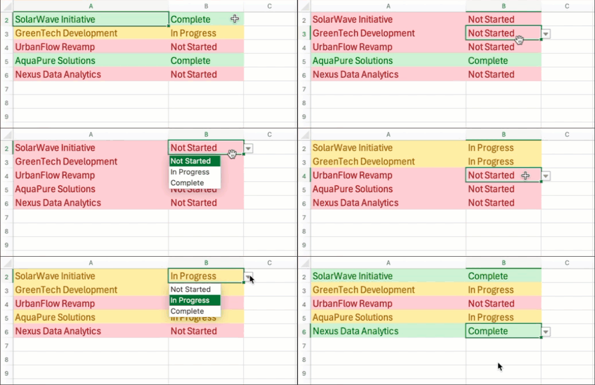
Now you’ll have improved data visibility, allowing you to spot important information more easily.
You can experiment with different colors and conditions to customize your spreadsheet to best fit your needs. The attachment below shows you the final Excel file with drop-down menus as well as the color coding that was performed in this article.